16:9 in English: Cutting and Film

By BARRY SALT

A very recent investigation into shot length patterns by James Cutting, Jordan DeLong, and Christine Nothelfer of Cornell University, has been published as Attention and the Evolution of Hollywood Films in the journal Psychological Science (fig. 1). This work by Cutting and his co-workers has attracted a lot of attention because it has been publicised as revealing the basic structure necessary for a film to be a commercial success. This is definitely not so, and the researchers do not make this claim themselves. Nevertheless, what they have to say is quite new enough to need discussion, which it is going to get here.

Over the last 90 years, a few people have occasionally tried to find significance of one kind or another in groups of shot lengths in films. After I introduced the concept of the Average Shot Length (ASL) of a film nearly forty years ago, as part of my project for the formal description of film style, which I called Statistical Style Analysis, I then looked at the variation from one scene to the next of the average shot length taken over the length of each scenes. The not very surprising result was that the average shot length did indeed vary from scene to scene, depending on the nature of the scene.

This happens because from the beginning of the 1920s onwards, the standard practice in American film making was that in writing a film script, the basic units of dramatic structure, which are the scenes, are put together so that the dramatic nature of successive scenes are contrasted. That is, in a typical film, a dialogue scene might be followed by an action scene, which might be followed by a comedy scene, which might be followed by another action scene, which is then followed by a romantic scene, and so on. At a slightly more basic level, this produces a “tension-release” pattern (or however you like to describe it), which is found in all traditional time-based arts, such as music, as well as in drama. And the two main varieties of film scenes are treated differently in their editing. Action scenes, and other dramatically tense ones, have fast cutting, and the other kinds have slower cutting to varying degrees. This in its turn follows standard notions about the expression of the content of a scene with the formal filmic devices used within it. “Long take” films, with an ASL of greater than 15 seconds, do not show these cutting rate variations so clearly. And action films made in the last few decades largely dispense with romantic scenes and comedy scenes, just retaining short slower cut dialogue scenes between the action, so the contrast in the cutting rates of successive scenes is now even more marked.

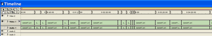
Nowadays, the way film-makers see the lengths of the shots in a film they are working on is as lengths marked down the timeline of a Non-linear Editing (an NLE) program such as Avid Media Composer or Final Cut Pro on the screen of a computer.

The timeline of a NLE program is not the ideal way to look at the succession of shot lengths in a film if one wants to study any large-scale patterns in them. A better way is to make a graph that plots the length of successive shots against their ordinal number down the length of the film. This could look like the following:

Here the shot lengths are measured in tenths of a second on the vertical axis, and the ordinal shot number is along the horizontal axis. Some years ago, Yuri Tsivian and Gunars Civjans invented a version of this with the vertical axis inverted, together with a software program to approximately measure the shot lengths in a film in real time, and they set up a web site dedicated to this approach, at www.cinemetrics.lv.

Their form of the shot length graph for The 39 Steps (1935) looks like this:

In the Cinemetrics graph, the ordinal shot number has been replaced by the point in the running time of the film at which a shot starts, so the horizontal axis is not scaled linearly in time. The red line is a first degree trendline, which shows that the cutting rate actually slows down over the length of the film.

A recent addition to the analytic features of Cinemetrics is a moving average. You can perhaps see in the above graph of the shot lengths in The 39 Steps that there are several clusters of long shots (20 seconds duration or more) alternating with short shots – for instance in the section from about 5 minutes to about 17 minutes. This particular stretch covers the scenes with the mysterious woman in Hannay’s (Robert Donat) flat up to his escape disguised as a milkman. Such sections alternate with stretches mostly made up of short shots only a few seconds long, for instance from 21 minutes to 25 minutes of the running time. This section covers the action scene on the train from Waverley station to Hannay’s escape on the Forth bridge. With the moving average added, which gives at each point the average shot length over 20 shots around any point, the graph looks like this:

This brings out the large scale variation in cutting rate down the length of the film, and incidentally picks out most of the scenes that make up the film.

The Cinemetrics site has flourished, and although the basic research approach to the large amount of data created on it is inductive, it has nevertheless revealed some large-scale regularities in patterns of shot lengths that would not have been detected otherwise.

Cutting Deeper

A statistical measure that has also been used in the past in the investigation of film structure by myself is the autocorrelation index. To understand this, consider the lengths of the first 31 of the 98 shots that make up the train scene just mentioned:

Now we can line them up with themselves shifted one to the right and drop the first number in the upper series:

The relationship of resemblance between these two series can be measured by calculating what is called the correlation coefficient, and in this particular case it is 0.046. A correlation coefficient of 0 means that there is no relation between the two series of numbers at all, while a correlation coefficient of 1 would mean that the two series were identical. So there is hardly any correlation between the two series. In this case, where we are comparing a series with itself, but shifted one place, the coefficient is referred to as an autocorrelation coefficient of lag one. If we move the lower series two places to the right, we get:

If we then repeat the calculation of the correlation coefficient, we now get an autocorrelation of lag 2, and it has the value of 0.38. This means that there is now a significant resemblance between the two series, even though this may not be very obvious to the eye. Up to this stage, we have been dealing with things that can be made fairly obvious visually, but now we have now reached a point where this is not so. And it is at this point that the research of Cutting, DeLong, and Nothelfer comes in.

What Cutting, DeLong and Nothelfer Did

The sample they worked with comprises 10 films from each of 15 years taken at five year intervals from 1935 to 2005: 10 films from 1935, 1940, 1945 and so forth. The sixty films from 1980 to 2005 that they use are said to be “…among the highest grossing of their year…”, and they are indeed near enough to the Top Ten box office champs for the years concerned. But for films chosen from before 1980, they chose films that “…were among those with the largest number of viewer ratings on the Internet Movie Database” (p. 2). It should be obvious to anybody acquainted with this source that such a choice cannot have a strong relationship with box office takings in that distant year in which these films were released. To give an example, their sample for 1945 (on the right) can be compared to the actual top ten US box-office films for that year (on the left).

Detour and Pursuit to Algiers are B-pictures, so they could not possibly have high box office listings for 1945, and likewise Brief Encounter, as even the best British films did not get general distribution in the US at that time.

Most importantly, if the desire was to test the hypothesis that the formula that the researchers arrived at was necessary for box office success, it is essential that the sample of highly successful films be compared with another sample of highly unsuccessful films, which should be shown to lack the formula. This was not done, as is so often the case in hypothesis testing in the softer sciences.

Attention in Cutting

Cutting et al. are concerned with investigating the occurrence of a hypothetical general pattern in human attention to sensory stimuli over time referred to as the 1/f pattern. At a basic level the 1/f pattern can be seen as a steady ebb and flow pattern. A more nuanced description is given by Cutting himself in a recent comment on cinemetrics.lv:

The 1/f pattern can be thought of as a simultaneous combination of many transverse, nonsynchronous waves whose up and down-ness, or amplitude (power is proportional to the square of the amplitude), is fixed by their wavelength (or the reciprocal of frequency, hence 1/f). Thus, the big (up and down) waves are also long waves (in time); smaller waves are shorter waves and proportionately so. For example, a relatively big wave might be exemplified by 60 consecutive shots that are relatively long followed by 60 shots that are relatively short, and with that pattern repeating; shorter and longer waves would also occur overlapping and within this original wave. (Cutting 2010)

Translated into the rhythm of film editing, an 1/f pattern would be the likely result of having shots “clustered in packets of shots of similar length” (p. 3), that is a steady fluctuation of, say, ten shots of 2-3 seconds followed by ten shots of 8-9 seconds. In their original article Cutting et al argue that “the rhythm of shot sequences in film is designed to drive the rhythm of attention and information uptake in the viewer” (p. 2), and their basic argument is that the closer the editing rhythm approximates the 1/f pattern the better it resonates with the rhythm of human attention.

There is some evidence for this particular 1/f pattern of attention, but it is far from confirmed at present, and even if it does exist as a general pattern, the neural mechanisms behind it are certainly unknown.

The research by Cutting, DeLong and Nothelfer suggests that the editing rhythm of recent Hollywood films has a closer fit with the 1/f pattern than films of the past (before 1980). This has led some commentators to the conclusion that they have found an editing formula for commercially successful films. Cutting and his co-workers do not make this claim but they do suggest that an 1/f editing pattern is more likely to appeal to audiences because the mind can be ’lost’ most easily with that editing structure (p. 7). Consequently, films with that editing pattern stand a better chance of being successful at the box office, and hence film-makers will tend to use these patterns more in editing films as time goes by.

Finer Detail

Cutting et al look for the 1/f pattern by using what is called Fourier analysis and also another technique called ARMA analysis. The varying lengths of shots as represented in one of the graphs above are obviously like a very irregular wave, and so the complete series for a film can be analysed as the result of the addition of multiple regular waves of varying frequency and amplitude using Fourier analysis. The resulting regular sine and cosine waves are characterised by their frequency and power. (Their power is proportional to their amplitude squared.) The result of this analysis is represented as a graph called a periodogram, like the one below for The 39 Steps.

In The 39 Steps, the power of the waves starts very high for low frequencies, and then rapidly declines to an approximately constant low level. The peaks of power decrease roughly as the reciprocal of the frequency, i.e. as 1/f, where “f” is the frequency. This is indicated by the blue line in the above graph. This sort of frequency spectrum is also referred to as “pink noise”. Measured at a power spectrum slope of 0.93, the editing of The 39 Steps is quite close to the 1/f pattern (see the supplemental material referred to earlier).

It is however, mixed with a lower level component of “white noise”, which is the sort of frequency spectrum in which the power of the frequencies that occur stays fairly constant across the range of frequencies. (This is indicated by the green line in the above graph.) Disentangling the two sets of frequencies is obviously a tricky business.

Contrast this with the periodogram for Sunset Boulevard (1950).

In this periodogram there is basically white noise alone. Cutting et al measure the editing pattern at a power spectrum slope of 0.26, as you can see in their supplemental material. The actual Cinemetrics graph representing the shot lengths in Sunset Boulevard reproduced below shows how there is not much obvious patterning in the sequence of shot lengths, compared with The 39 Steps. That is, there is no sign of the stretches of nearly equal fast cut shots seen in The 39 Steps.

The method that Cutting et al. use for their detailed frequency analysis goes through a series of complicated stages that you can read in their original article.

They also use another form of analysis called autoregression, which is a more complicated development of the kind of autocorrelation analysis that I demonstrated above. This autoregression analysis produces an autoregression index, AR, which has integral values, and then, after further steps, a modified autoregression index mAR. The latter gives somewhat similar results to their frequency analysis, but not identical ones. This is a little worrying, since the two methods are directly related mathematically, by the Wiener–Khinchin theorem, so one would expect their results to be more or less identical, whereas discrepancies exist between the two methods right across the range of values, and not just at higher end, as they suggest.

What Happened in History

The historical part of the phenomenon we are talking about is the increase in the cutting rate since the nineteen-forties. This is illustrated by a graph covering the Average Shot Lengths of 7,448 American films made between 1930 and 2006, which is in the new 3rd. edition of my Film Style and Technology on page 378. This increase has certainly been consciously intentional on the part of the film-makers over the last thirty years.

Now I am not suggesting that the increase in the cutting rate since the nineteen-forties directly causes the phenomenon that Cutting and co-workers have studied, but I am suggesting that the speed-up in cutting has caused other things, that in their turn cause the Cutting phenomenon.

As I understand it, the nub of the matter is that the increase in the autoregression indices, AR and mAR, and in the slope of the 1/f measure in Fourier decomposition of shot lengths, results from having more strings of roughly equal length shots in a film.

These strings of roughly equal length shots occur mainly in action scenes, but also in scenes edited to music, either in dramatic films, or in actual musicals. (Anchors Aweigh (1945), The Sound of Music (1965) and Popeye (1980) are actually musicals, not simple comedies, as they are listed by Cutting et al.) The trend towards the increase in the mAR indices and 1/f slope comes from having more of the running time of an action film devoted to action scenes. There has also been a trend towards editing action scenes to a pre-existing music track, either a dummy one, or the actual piece of pop music that is going to be used in the final sound track, which also helps the effect.

Editors have more rushes to deal with nowadays for two reasons. More shots are taken so that an increased cutting rate is possible for the film, and as part of that, more “coverage” is shot. (“Coverage” is more shots of the same action taken from different angles.) Many of the Hollywood directors of the classical period prided themselves on “cutting in the camera” – i.e. only taking the shots they knew would be needed in the final cut. One does not hear that sort of boast any longer. So this current situation does give editors a bit more freedom about the lengths of shot they use. But not in ordinary dramas, where the length of the lines of dialogue strongly influence the shot lengths.

Cutting, DeLong and Nothelfer give the impression that the editor of a film has complete freedom to make a shot any length they like. This is certainly not the case in general, as anyone who has edited a film knows. In particular, for dialogue scenes, the length of the speeches has a strong influence on shot length. Even when there are cutaways to reaction shots in the middle of a speech, these tend to follow the length of sentences within the individual speeches. There is more freedom for an editor to choose shot length in action scenes, but the need for cuts on action at certain points again exerts some control on shot length, and even the length of the actions of the actors themselves, as staged, has to be respected.

It is these and other independent causes simultaneously acting to determine the lengths of shots that produce the usual Lognormal distribution of shot lengths, as I have said so often before. However, the trend towards using more jump cuts within scenes, which is demonstrated in the “Statistical Style Analysis – Part 4” section of my Film Style and Technology: History and Analysis (3rd edition), does give some more freedom to choose the shot length independently of the content of the shot, if editors want to. This freedom is inherent in a montage sequence, and accounts for the very large chains of similar length shots in Rocky IV (1985), as revealed in the analysis by Cutting and his co-workers. Rocky IV has many (too many) training montage sequences cut to the regular beat of music, which is what pushes it right up to the top of the shot correlation stakes. If audiences could be satisfied with nothing but action movies that have NOTHING but action in them, then the ASL could get shorter than the minimum of 1.5 seconds, where it has halted at present, and the various shot length correlations studied by Cutting et al. could attain the maximum all the time, but I don’t think this is likely.

On the Large Scale

James Cutting has more recently suggested that the long waves measure the location of “Acts” in the film structure, but this seems dubious to me, since I don’t believe that film scripts are actually constructed in terms of “Acts”. I think most films script-writers don’t believe in “Act” divisions either. The act concept is indeed used by some film producers and directors in discussing scripts, and of course by non-script writers writing books about how to write film scripts. Anyway, this hypothesis can be tested by using the Fourier transform method to see whether it gives locations for act boundaries that coincide with those postulated in a particular film by someone who believes in them, such as Kristin Thompson.

There are some further doubts about the postulated fundamental connection between the (hypothetical) basic psychological processes of attention, and film shot lengths. One alternative view of the matter is that the film audience is primarily attending to the succession of things represented in the film scenes, not the cuts between the shots. These cuts were certainly intended by film-makers to be “invisible” up until recent times. The counter-example to think about here is the most popular variety of videogame, while also remembering that videogames make more money than films nowadays. This is the “first person shooter”, which consists of just a continuous Point of View shot of what is meant to be in the protagonist’s sight, with no cuts in the scene shown on the computer screen. In first person shooters the player’s attention is totally gripped, completely without the benefit of editing.
Another thing about Cutting et al.’s ideas that still bothers me is the question, “Why are films mostly still falling short of the maximum mAR and 1/f slope after 90 years of the use of standard film construction, if the postulated psychological effect is so powerful?”

Nevertheless, all the above is obviously far from being the last word on this work by Cutting et al., and what they have done is certainly usefully provocative.